PID Controllers Explained

A PID controller—Proportional-Integral-Derivative—is a key element in industrial process control. By continuously comparing a measured process variable to a target setpoint, the PID controller calculates and applies adjustments based on three terms (proportional, integral, and derivative). This feedback approach enables accurate and stable regulation of parameters like temperature, pressure, and motor speed. Below, we break down the PID controller’s components, how it is tuned, common challenges, and some of its most prevalent applications.

1. Core PID Elements

1.1 Proportional (P)

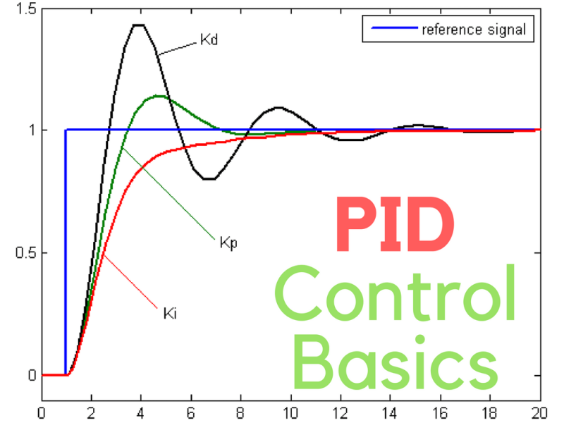
The P-term produces an output proportional to the real-time error (the difference between the setpoint and the measured value). The proportional gain, Kp, determines how aggressively the controller reacts. If Kp is too large, the system may oscillate. If it is too small, the system might respond slowly or incur steady-state error.

1.2 Integral (I)

The I-term accumulates the error over time and eliminates residual offset. By integrating past errors, it compensates for any persistent difference between the setpoint and actual value. The integral gain, Ki, governs the speed of this accumulation. Excessive integral gain can cause overshoot or oscillations, while insufficient gain prolongs the correction of offset errors.

1.3 Derivative (D)

The D-term anticipates future error by reacting to the rate of change (slope) of the error signal. By applying a corrective action proportional to how quickly the error is shifting, the derivative gain, Kd, can reduce overshoot. However, high derivative gain makes the controller sensitive to noise.

2. Mathematical Overview

A PID controller calculates the control output $u(t)$ as follows:

$$u(t) = K_p \cdot e(t) + K_i \cdot \int e(t) \,dt + K_d \cdot \frac{d e(t)}{d t}$$

where:

• $e(t)$ = difference between setpoint and actual process value
• $K_p$, $K_i$, $K_d$ = proportional, integral, and derivative gains

3. Tuning a PID Controller

3.1 Ziegler–Nichols Method

A classic approach involves:

1. Disable I and D: Keep only the P term active.
2. Increase $K_p$ Until Sustained Oscillations: Adjust until the system oscillates steadily.
3. Identify Critical Gain and Oscillation Period: Label these parameters.
4. Apply Ziegler–Nichols Formulas: Calculate $K_p$, $K_i$, and $K_d$ from standard tables or guidelines.

Although effective for initial tuning, Ziegler–Nichols often requires refinements to suit specific performance criteria.

3.2 Manual Tuning

An alternative is trial-and-error:

1. Set All Gains to Zero: Begin from a baseline.
2. Increment $K_p$: Achieve a reasonable response.
3. Add $K_i$: Remove steady-state error.
4. Add $K_d$: Reduce overshoot or oscillations if necessary.

4. Practical Tips

• Start Small: Begin with low gain values to prevent instability and observe system behavior.
• Balance Speed vs. Overshoot: High gains offer quick responses but risk oscillation.
• Account for Noise: Excessive derivative gain may amplify measurement noise.
• Consider System Constraints: Some processes handle more aggressive changes than others.

5. Common Issues and Solutions

5.1 System Oscillations

If the loop oscillates, reduce the proportional gain or adjust the integral/derivative terms. Too high a gain triggers rapid responses that cause instability.

5.2 Slow Response

For a sluggish system, raise Kp or increase Ki to help reduce offset faster. But do so carefully to avoid overshoot.

5.3 Overshoot

Excessive overshoot can be minimized by adding or increasing derivative action (Kd) or by lowering proportional gain.

6. Real-World Applications

6.1 Industrial Processes

PID controllers are integral to:

• Temperature Control: Boilers, ovens, and chemical reactors.
• Pressure Regulation: Pipelines, hydraulic systems, and compressors.
• Motor Speed Control: Servo systems and conveyor lines.
• Fluid Level Management: Tanks, sumps, and open-channel flow control.

6.2 Robotics

In robotics, PID controllers drive:

• Servo Positioning: Joint control in robotic arms.
• Speed Regulation: Smooth transitions and stable velocities.
• Balancing and Stabilization: Two-wheeled robots, drones, or self-balancing vehicles.

7. Evolving Trends and Outlook

7.1 Adaptive and Self-Tuning

Modern control systems are adopting adaptive PID controllers that automatically adjust gains to changing process conditions. This adaptive approach maintains optimal performance despite parameter drift or load variations.

7.2 Digital Implementation

Most PID controllers today are software-based (e.g., in programmable logic controllers or embedded microcontrollers). Key benefits include:

• Easy Parameter Adjustments: Gains can be modified at runtime.
• Advanced Functions: Additional logic layers or safety checks.
• Remote Configuration: Networked devices allow for off-site tuning.

Conclusion

A PID controller remains one of the most widely used and effective control strategies, offering a blend of simplicity and robust performance. By combining proportional, integral, and derivative actions, it addresses steady-state errors while controlling overshoot and response speed.

Success hinges on careful tuning and an understanding of the process’s unique dynamics. With digital implementations, system integrators gain flexibility to refine PID parameters and tailor advanced control features. From chemical plants and HVAC systems to robotics, PID control remains a cornerstone of efficient, stable, and high-precision automation.

At safsale.com, we recognize that mastering PID tuning is an essential step for anyone working in modern engineering. Whether you’re refining industrial lines or perfecting robotic control loops, a well-tuned PID solution can drastically enhance productivity and maintain stable, high-performance operations.